![]()
The gbfs package supplies a set of functions to interface with General Bikeshare Feed Specification .json feeds in R, allowing users to save and accumulate tidy .rds datasets for specified cities/bikeshare programs. The North American Bikeshare Association’s gbfs is a standardized data release format for live information on the status of bikeshare programs, as well as metadata, including counts of bikes at stations, ridership costs, and geographic locations of stations and parked bikes.
Features
- Get bikeshare data by specifying city name or supplying url of feed
- All feeds for a city can be saved with a single function
- New information from dynamic feeds can be appended to existing datasets
Installation
We’re on CRAN! Install the latest release with:
install.packages("gbfs")
library(gbfs)
You can install the developmental version of gbfs from GitHub with:
# install.packages("devtools")
devtools::install_github("simonpcouch/gbfs")
Background
The gbfs is a standardized data feed describing the current status of a bikeshare program.
Although all of the data is live, only a few of the datasets change often:
-
station_status: Supplies the number of available bikes and docks at each station as well as station availability -
free_bike_status: Gives the coordinates and metadata on available bikes that are parked, but not at a station.
In this package, these two datasets are considered “dynamic”, and can be specified as desired datasets by setting feeds = "dynamic" in the main wrapper function in the package, get_gbfs.
Much of the data supplied in this specification can be considered static. If you want to grab all of these for a given city, set feeds = "static" when calling get_gbfs. Static feeds include:
-
system_information: Basic metadata about the bikeshare program -
station_information: Information on the capacity and coordinates of stations - Several optional feeds:
system_hours,system_calendar,system_regions,system_pricing_plans, andsystem_alerts
Each of the above feeds can be queried with the get_suffix function, where suffix is replaced with the name of the relevant feed.
For more details on the official gbfs spec, see this document.
Example
In this example, we’ll grab data from Portland, Oregon’s Biketown bikeshare program and visualize some of the different datasets.
First, we’ll grab some information on the stations.
# grab portland station information and return it as a dataframe
pdx_station_info <-
  get_station_information("https://gbfs.lyft.com/gbfs/1.1/pdx/gbfs.json")
#> Message: Returning the output data as an object, rather than saving it, since the `directory` argument was not specified. Setting `output = "return"` will silence this message.

# check it out!
glimpse(pdx_station_info)
#> Rows: 165
#> Columns: 19
#> $ region_code                          <chr> "biketown_pdx", "biketown_pdx", "biketown_pdx", "biketown_pdx", "PDX…
#> $ legacy_id                            <chr> "1440914125193298376", "14409138…
#> $ station_type                         <chr> "lightweight", "lightweight", "l…
#> $ eightd_station_services              <list> [[], [], [], [], [], [], [], []…
#> $ external_id                          <chr> "motivate_PDX_144091412519329837…
#> $ lon                                  <dbl> -122.6813, -122.6687, -122.6604,…
#> $ has_kiosk                            <lgl> FALSE, FALSE, FALSE, FALSE, FALS…
#> $ name                                 <chr> "SW Yamhill at Director Park", "…
#> $ station_id                           <chr> "1440914125193298376", "14409138…
#> $ dockless_bikes_parking_zone_capacity <int> 20, 12, 18, 18, 6, 10, 6, 12, 18…
#> $ capacity                             <int> 20, 12, 18, 18, 6, 10, 6, 12, 18…
#> $ lat                                  <dbl> 45.51898, 45.53480, 45.55645, 45…
#> $ rack_model                           <chr> "CITY_PILOT_RACK", "CITY_PUBLIC_…
#> $ address                              <chr> "Park Avenue West, Southwest Yam…
#> $ eightd_has_key_dispenser             <lgl> FALSE, FALSE, FALSE, FALSE, FALS…
#> $ electric_bike_surcharge_waiver       <lgl> FALSE, FALSE, FALSE, FALSE, FALS…
#> $ client_station_id                    <chr> "motivate_PDX_144091412519329837…
#> $ rental_uris.ios                      <chr> "https://pdx.lft.to/lastmile_qr_…
#> $ rental_uris.android                  <chr> "https://pdx.lft.to/lastmile_qr_…
…as well as the number of bikes at each station.
# grab current capacity at each station and return it as a dataframe
pdx_station_status <-
  get_station_status("https://gbfs.lyft.com/gbfs/1.1/pdx/gbfs.json")
#> Message: Returning the output data as an object, rather than saving it, since the `directory` argument was not specified. Setting `output = "return"` will silence this message.

# check it out!
glimpse(pdx_station_status)
#> Rows: 165
#> Columns: 19
#> $ is_renting                <int> 1, 1, 1, 1, 1, 1, 1, 1, 1, 1, 1, 1, 1, 1, 1…
#> $ station_id                <chr> "1440914030704017724", "1440914074618217706…
#> $ is_installed              <int> 1, 1, 1, 1, 1, 1, 1, 1, 1, 1, 1, 1, 1, 1, 1…
#> $ num_docks_available       <int> 9, 5, 4, 8, 18, 8, 2, 4, 17, 12, 11, 5, 17,…
#> $ num_docks_disabled        <int> 0, 0, 0, 0, 0, 0, 0, 0, 0, 0, 0, 0, 0, 0, 0…
#> $ is_returning              <int> 1, 1, 1, 1, 1, 1, 1, 1, 1, 1, 1, 1, 1, 1, 1…
#> $ last_reported             <dbl> 1.599610e+12, 1.599610e+12, 1.599610e+12, 1…
#> $ num_ebikes_available      <int> 9, 6, 7, 7, 0, 6, 5, 1, 1, 5, 7, 7, 1, 2, 3…
#> $ num_bikes_available       <int> 0, 0, 0, 0, 0, 0, 0, 0, 0, 0, 0, 0, 0, 0, 0…
#> $ eightd_has_available_keys <lgl> FALSE, FALSE, FALSE, FALSE, FALSE, FALSE, F…
#> $ station_status            <chr> "active", "active", "active", "active", "ac…
#> $ legacy_id                 <chr> "1440914030704017724", "1440914074618217706…
#> $ num_bikes_disabled        <int> 0, 0, 0, 0, 0, 0, 0, 0, 0, 0, 0, 0, 0, 0, 0…
#> $ last_updated              <dttm> 2020-10-04 12:44:55, 2020-10-04 12:44:55, …
#> $ year                      <dbl> 2020, 2020, 2020, 2020, 2020, 2020, 2020, 2…
#> $ month                     <dbl> 10, 10, 10, 10, 10, 10, 10, 10, 10, 10, 10,…
#> $ day                       <int> 4, 4, 4, 4, 4, 4, 4, 4, 4, 4, 4, 4, 4, 4, 4…
#> $ hour                      <int> 12, 12, 12, 12, 12, 12, 12, 12, 12, 12, 12,…
#> $ minute                    <int> 44, 44, 44, 44, 44, 44, 44, 44, 44, 44, 44,…
Just like that, we have two tidy datasets containing information about Portland’s bikeshare program.
Joining these datasets, we can get the capacity at each station, along with each station’s metadata.
# full join these two datasets on station_id and select a few columns
pdx_stations <- full_join(pdx_station_info,
                          pdx_station_status,
                          by = "station_id") %>%
  # just select columns we're interested in visualizing
  select(id = station_id,
         lon,
         lat,
         num_bikes_available,
         num_docks_available) %>%
  mutate(type = "docked")
Finally, before we plot, lets grab the locations of the bikes parked in Portland that are not docked at a station,
# grab data on free bike status and save it as a dataframe
pdx_free_bikes <-
  get_free_bike_status("https://gbfs.lyft.com/gbfs/1.1/pdx/gbfs.json",
                       output = "return") %>%
  # just select columns we're interested in visualizing
  select(id = bike_id, lon, lat) %>%
  # make columns analogous to station_status for row binding
  mutate(num_bikes_available = 1,
         num_docks_available = NA,
         type = "free")
…and bind these dataframes together!
# row bind stationed and free bike info
pdx_full <- bind_rows(pdx_stations, pdx_free_bikes)
Now, plotting,
# filter out stations with 0 available bikes
pdx_plot <- pdx_full %>%
  filter(num_bikes_available > 0) %>%
  # plot the geospatial distribution of bike counts
  ggplot() +
  aes(x = lon,
      y = lat,
      size = num_bikes_available,
      col = type) +
  geom_point() +
  # make aesthetics slightly more cozy
  theme_minimal() +
  scale_color_brewer(type = "qual")
pdx_plot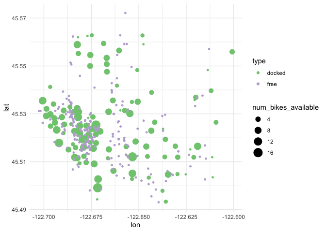
Folks who have spent a significant amount of time in Portland might be able to pick out the Willamette River running Northwest/Southeast through the city. With a few lines of gbfs, dplyr, and ggplot2, we can put together a meaningful visualization to help us better understand how bikeshare bikes are distributed throughout Portland.
Some other features worth playing around with in gbfs that weren’t touched on in this example:
- The main wrapper function in the package,
get_gbfs, will grab every dataset for a given city. (We call the functions to grab individual datasets above for clarity.) - In the above lines, we output the datasets as returned dataframes. If you’d rather save the output to your local files, check out the
directoryandreturnarguments. - When the
outputargument is left as default inget_free_bike_statusandget_station_status(the functions for thedynamicdataframes,) and a dataframe already exists at the given path,gbfswill row bind the dataframes, allowing for the capability to accumulate large datasets over time. - If you’re not sure if your city supplies
gbfsfeeds, you might find theget_gbfs_citiesandget_which_gbfs_feedsfunctions useful.
Contributing
Please note that the gbfs R package is released with a Contributor Code of Conduct. By contributing to this project, you agree to abide by its terms.